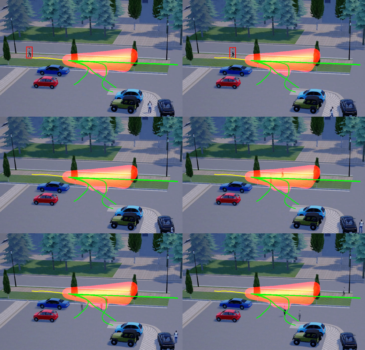
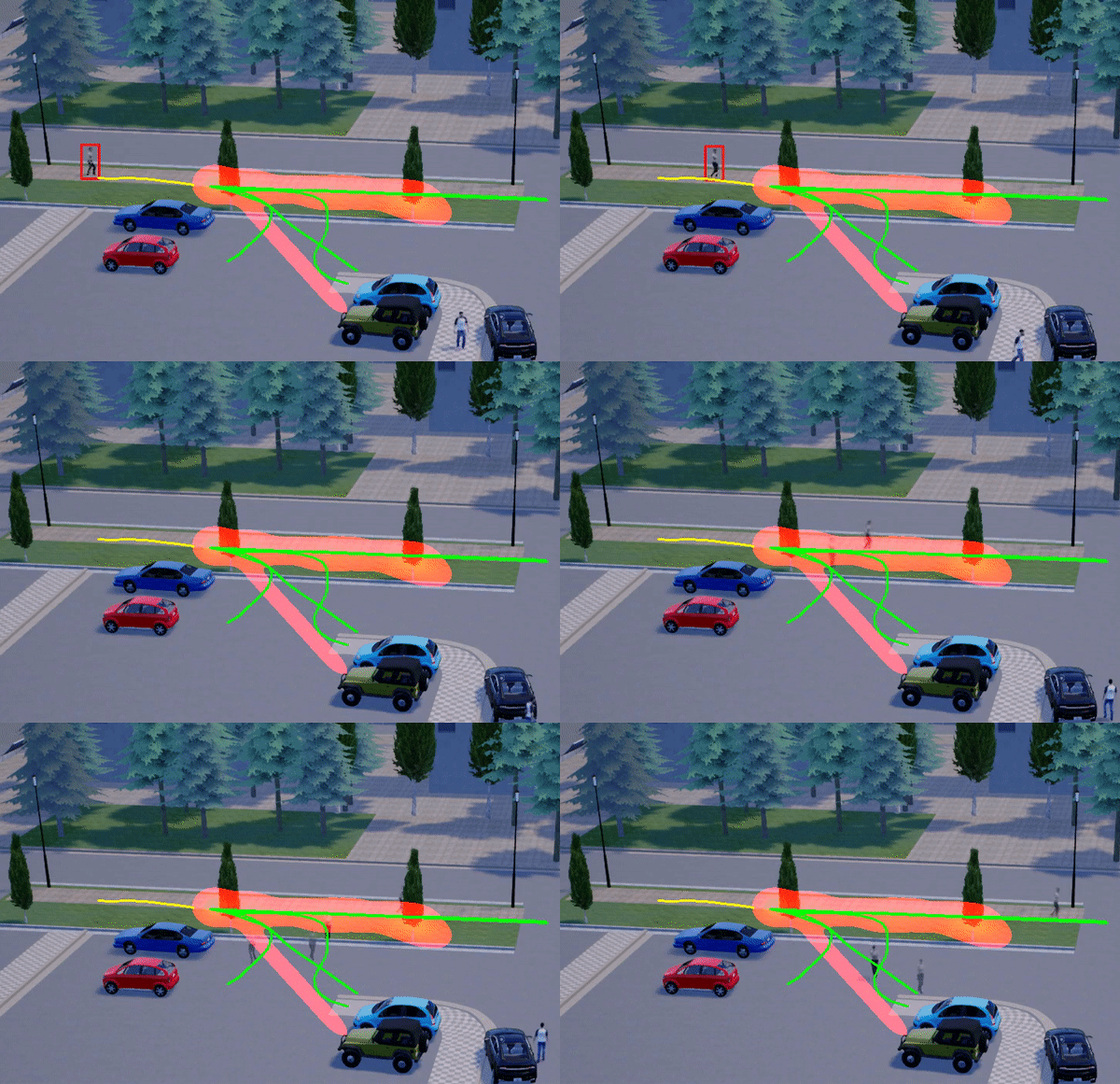
## Single Future Trajectory Prediction
We experimented on the [ActEv dataset](https://actev.nist.gov) by following the [Next-prediction](https://github.com/google/next-prediction) evaluation protocol.
First download the processed annotations from the [Next-prediction](https://github.com/google/next-prediction) repo.
```
$ wget https://precognition.team/next/data/072019_prepare_data/072019_next_my_prepare_nopersoncnn.tgz
$ tar -zxvf 072019_next_my_prepare_nopersoncnn.tgz
```

Then download pretrained models by running the script
`bash scripts/download_single_models.sh`.

### Step 1: Preprocess
Preprocess the data for training and testing.
The following is for ActEv experiments.

```
$ python code/preprocess.py prepared_data/traj_2.5fps/ actev_preprocess \
--obs_len 8 --pred_len 12 --add_kp --kp_path prepared_data/anno_kp/ \
--add_scene --scene_feat_path prepared_data/actev_all_video_frames_scene_seg_every30_36x64/ \
--scene_map_path prepared_data/anno_scene/ --scene_id2name prepared_data/scene36_64_id2name_top10.json \
--scene_h 36 --scene_w 64 --video_h 1080 --video_w 1920 --add_grid \
--add_person_box --person_box_path prepared_data/anno_person_box/ \
--add_other_box --other_box_path prepared_data/anno_other_box/ \
--add_activity --activity_path prepared_data/anno_activity/ \
--person_boxkey2id_p prepared_data/person_boxkey2id.p --add_all_reg
```

### Step 2: Test the model
Run testing with our pretrained single model for ActEv experiments.
```
$ python code/test.py actev_preprocess multiverse-models multiverse_single18.51_multi168.9_nll2.6/ \
--wd 0.001 --runId 0 --obs_len 8 --pred_len 12 --emb_size 32 \
--enc_hidden_size 256 --dec_hidden_size 256 --activation_func tanh \
--keep_prob 1.0 --num_epochs 80 --batch_size 16 --init_lr 0.01 --use_gnn \
--use_scene --learning_rate_decay 0.95 --num_epoch_per_decay 2.0 \
--grid_loss_weight 1.0 --grid_reg_loss_weight 0.1 --save_period 500 \
--scene_h 36 --scene_w 64 --scene_conv_kernel 3 --scene_conv_dim 64 \
--scene_grid_strides 2,4 --use_grids 1,0 --val_grid_num 0 --gpuid 0 --load_best
```

The evaluation result should be:
<table>
  <tr>
    <td>ADE</td>
    <td>FDE</td>
  </tr>
  <tr>
    <td>18.51</td>
    <td>35.84</td>
  </tr>
</table>

Test the model trained on simulation videos (anchor videos) only:
```
$ python code/test.py actev_preprocess multiverse-models multiverse_simtrained_single22.9/ \
--wd 0.001 --runId 0 --obs_len 8 --pred_len 12 --emb_size 32 \
--enc_hidden_size 256 --dec_hidden_size 256 --activation_func tanh \
--keep_prob 1.0 --num_epochs 80 --batch_size 16 --init_lr 0.01 --use_gnn \
--use_scene --learning_rate_decay 0.95 --num_epoch_per_decay 2.0 \
--grid_loss_weight 1.0 --grid_reg_loss_weight 0.1 --save_period 500 \
--scene_h 36 --scene_w 64 --scene_conv_kernel 3 --scene_conv_dim 64 \
--scene_grid_strides 2,4 --use_grids 1,0 --val_grid_num 0 --gpuid 0 --load_best
```

The evaluation result should be:
<table>
  <tr>
    <td>ADE</td>
    <td>FDE</td>
  </tr>
  <tr>
    <td>22.94</td>
    <td>43.34</td>
  </tr>
</table>


## Multi-Future Trajectory Prediction
In this section we show how to do multi-future trajectory inferencing on the Forking Paths dataset. First follow instructions [here](forking_paths_dataset/README.md#prepare-data) to prepare the data.

Suppose you have the data prepared in the `forking_paths_dataset` folder. Run multi-future inferencing by:
```
$ python code/multifuture_inference.py forking_paths_dataset/next_x_v1_dataset_prepared_data/obs_data/traj_2.5fps/test/ \
forking_paths_dataset/next_x_v1_dataset_prepared_data/multifuture/test/ \
multiverse-models/multiverse_single18.51_multi168.9_nll2.6/00/best/ \
model1_output.traj.p --save_prob_file model1_output.prob.p \
--obs_len 8 --emb_size 32 --enc_hidden_size 256 --dec_hidden_size 256 \
--use_scene_enc --scene_id2name prepared_data/scene36_64_id2name_top10.json \
--scene_feat_path forking_paths_dataset/next_x_v1_dataset_prepared_data/obs_data/scene_seg/ \
--scene_h 36 --scene_w 64 --scene_conv_kernel 3 --scene_conv_dim 64 \
--grid_strides 2,4 --use_grids 1,0 --num_out 20 --diverse_beam --use_gnn \
--diverse_gamma 0.01 --fix_num_timestep 1 --gpuid 0
```

This will save the trajectory output to `model1_output.traj.p` and grid probabilities to `model1_output.prob.p`.
To evaluate trajectories using minADE/minFDE metrics:
```
$ python code/multifuture_eval_trajs.py forking_paths_dataset/next_x_v1_dataset_prepared_data/multifuture/test/ \
model1_output.traj.p
```

The evaluation result should be:
<table>
  <tr>
    <td>45-degree-ADE</td>
    <td>top-down-ADE</td>
    <td>45-degree-FDE</td>
    <td>top-down-FDE</td>
  </tr>
  <tr>
    <td>169.96</td>
    <td>158.90</td>
    <td>336.25</td>
    <td>318.40</td>
  </tr>
</table>

To evaluate using Negative Log-Likelihood metric:
```
$ python code/multifuture_eval_trajs_prob.py forking_paths_dataset/next_x_v1_dataset_prepared_data/multifuture/test/ \
model1_output.prob.p
```

The evaluation result should be:
<table>
  <tr>
    <td>T=1</td>
    <td>T=2</td>
    <td>T=3</td>
  </tr>
  <tr>
    <td>2.63</td>
    <td>5.43</td>
    <td>10.21</td>
  </tr>
</table>

## Visualization
To visualize the model output, follow [this](forking_paths_dataset/README.md#visualize-the-dataset) to generate multi-future videos, and then run:
```
$ python code/vis_multifuture_trajs_video.py forking_paths_dataset/next_x_v1_dataset_prepared_data/multifuture/test/ \
model1_output.traj.p forking_paths_dataset/multifuture_visualization/ \
model_output_visualize_videos --show_obs --use_heatmap --drop_frame 10
$ cd model_output_visualize_videos
$ for file in *;do ffmpeg -framerate 4 -i ${file}/%08d.jpg ${file}.mp4;done
```

<div align="center">
  <div style="">
      <img src="images/0400_40_256_cam2_sgan.gif" height="255px" />
      <img src="images/0400_40_256_cam2_ours.gif" height="255px" />
  </div>
  <p style="font-weight:bold;font-size:1.2em;">
    Qualitative analysis between Social-GAN (left) and our model.
  </p>
</div>